The Cycloid and Other Curves

Parametrized curves occur in a number of different settings and in a variety of applications. For example, the cycloid is the path traced out by a point on a wheel as it rolls on a horizontal surface. (Click image below to animate)

In particular, suppose that R is the radius of a wheel rolling along the x -axis, and suppose that the point on the wheel that traces out the cycloid is at (0,0) initially. If the wheel rotates through an angle , then it rolls a distance R along the x -axis.

As a result, if the point (0,0) is moved to the point ( x,y ) by the rolling of the wheel, then

x + R = R , y + R = R

so that

x = , y =

Moreover, if the wheel is rolling with an angular speed of radians per unit time and if t denotes time, then the angle is related to the time t by . As a result, the parametrization of the cycloid is

x = , y =

which as a vector-valued function is

r ( t ) = [ , ]

Let's draw this curve along with the circle and point that traces it out. First we define the curve.

> R:=2; # radius of the wheel
omega:=1; # angular velocity of the wheel in units of radians per unit time
cycloid:=[R*omega*t-R*sin(omega*t),R-R*cos(omega*t)];

>

Next, we draw the cycloid in grey, then retrace it in blue. We include the circle and the point P for illustration.

> min_t:=0: #Enter the low value of the parameter
max_t:=5*Pi: #Enter the high value of the parameter
cycloid_static:=plot([cycloid[1],cycloid[2],t=min_t..max_t],color=grey):
for i from 1 to 30 do # Draw 30 frames to be displayed in sequence
current_t:=min_t+max((i-1)*(max_t-min_t)/30,0.01):
wheel:=circle([R*omega*current_t,R],R,color=brown):
P_point:=disk(subs(t=current_t,cycloid),0.3,color=black):
P_label:=textplot([subs(t=current_t,cycloid[1])-0.4,
subs(t=current_t,cycloid[2])+0.4,`P`],font=[TIMES,ITALIC,12],align={ABOVE,LEFT}):
cycloid_sec:=plot([cycloid[1],cycloid[2],t=min_t..current_t],color=blue):
cyc_frames[i]:=display(wheel,P_point,cycloid_sec):
end do:
cycloid_ani:=display([seq(cyc_frames[i],i=1..30)],insequence=true):
display(cycloid_static,cycloid_ani,scaling=constrained);

>

Circles are often used to form more elaborate curves, as is evidenced by the once popular children's toy Spirograph. In particular, many interesting curves can be formed by rolling a smaller circle on the inside of a larger circle, or alternatively, by rolling any circle on the outside of another circle. For example, let's define a curve by following the path of a point P on the edge of a circle of radius 1/4 as it rolls on the inside of the unit circle.

Once the smaller circle has rolled through an angle , the center of the smaller circle is at ( ). Moreover, if the smaller circle rolls without slipping, then the green and blue arcs must have the same length. The relationship implies that the smaller circle has rotated through an angle of .

Thus, P is at the point offset from the center by the sine and cosine of , which is at

( cos( ) + cos( ), sin( ) + sin( ) )

However, identifies for triple angles reduce these even further:

> 1/4*cos(3*theta)=expand(1/4*cos(3*theta));
3/4*cos(theta)+1/4*cos(3*theta)=expand(3/4*cos(theta)+1/4*cos(3*theta));

>

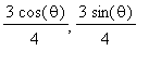
Likewise, the y -coordinates simplify, thus implying that the coordinates of P are

( ( ), ( ) )

Since P traces out the astroid, the parametrization of the astroid is

r ( t ) = [ ( t ), ( t ) ]

Let's look at the astroid graphically below:

> min_t:=0: max_t:=2*Pi: #Once around the circle
unitcircle:=plot([cos(t),sin(t),t=0..2*Pi],color=black):
for i from 1 to 30 do # Draw 30 frames to be displayed in sequence
current_t:=min_t+max((i-1)*(max_t-min_t)/29,0.01):
innercircle:=circle([0.75*cos(current_t),0.75*sin(current_t)],0.25,color=brown):
astroid:=plot([cos(t)^3,sin(t)^3,t=0..current_t],color=blue):
P_point:=disk([cos(current_t)^3,sin(current_t)^3],0.02,color=black):
P_label:=textplot([0.9*cos(current_t)^3,0.9*sin(current_t)^3,`P`],
font=[TIMES,ITALIC,12],align={BELOW,LEFT}):
cyc_frames[i]:=display(innercircle,astroid,P_point,P_label):
end do:
cycloid_ani:=display([seq(cyc_frames[i],i=1..30)],insequence=true):
display(unitcircle,cycloid_ani,scaling=constrained);

>