Exercises
-
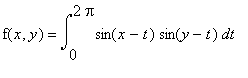
1. Define the function
f
(
x,y
) =
 using both the arrow and the unapply methods. Then use both to evaluate

-
2. Suppose we wanted to define the function
-
-
How would the use of the arrow differ from the use of the unapply command?
-
3. The integral
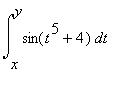 cannot be evaluated in closed form. Suppose we want to define the function
-
f
(
x,y
) =

-
so that each time a point (
x,y
) is input, a numerical approximation of the resulting integral is returned. What Maple command structure would accomplish this task? (Hint: to numerically evaluate an integral, simply place the int() command within an evalf() command. For example, evalf(int(x^3,x=0..1)) will numerically integrate x^3 from 0 to 1).
-
4. Graph the function
f
(
x,y
) =
 over the region
x
=-1..1,
y=
-1..1 and also over the region on and inside the unit circle. Explain why the two graphs do not look the same.
over the region
x
=-1..1,
y=
-1..1 and also over the region on and inside the unit circle. Explain why the two graphs do not look the same.
-
5. For
x
from -5 to 5 and for
t
from 0 to 10, animate the slices of
-
u
(
x,t
) =

-
Then graph the surface
z
=
u
(
x,t
) and show the slices as
t
increases from 0 to 0.
-
6. What is going on in the following animation of
u
(
x,t
) = sin(
x-t
)? Can you reproduce the Maple commands used to produce it? (Click and play the figure below):
![[Maple Plot]](images/2-122.gif)
-
-
7. The animation in
t
of the function
u
(
x,t
)
=
sin(
x-t
)+sin(
x+ t
) is called a
bidirectional wave
. What happens if you "follow" a point on the wave as the animation in exercise 6 does? For fixed
t
, what is the tangent line to
y = u
(
x,t
) at
x=
0? Animate a short section of the tangent line along with an animation of the original function.
-
8. In the animation below we see a region in the
xy
-plane being deformed into the graph of a function
z
=
f
(
x,y
) over that region.
![[Maple Plot]](images/2-123.gif)
-
What sequence of
Maple
commands could you use to produce this animation?
-