Constrained Optimization
In many applications, we must find the extrema of a function f(x,y) subject to a constraint, where a constraint is a curve
of the form
Such problems are called constrained optimization problems.
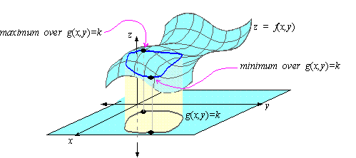
Geometrically, constrained optimization is the problem of finding the points
on the curve g( x,y) = k for which f( x,y) attains
it largest and smallest values.
In particular, when g( x,y) = k is a closed curve parametrized
by r( t) =
á x( t) ,y(t)
ñ for t in [ a,b] , then the absolute
extrema of f( x,y) subject to g( x,y) = k must
occur at the critical points of z( t) = f( x( t),y( t) ) .
Moreover, if g( x,y) = k and f( x,y) are both
smooth, then the critical points of z( t) are the solutions to
where v is the velocity of r( t) . That is,
the critical points of z( t) occur when Ńf^v. And since Ńg^v, it follows that the extrema of f( x,y) subject to g( x,y) = k occur when Ńf
is parallel to Ńg.Let's view this in a different way. Let's suppose that as the levels of f( x,y)
increase, short sections of level curves of f( x,y) form
secant curves to g( x,y) = k
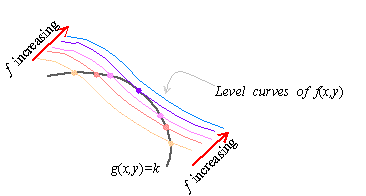
It follows that the highest level curve of f( x,y) intersecting g(x,y) = k must be tangent to the curve g( x,y) = k, which
is possible only if their gradients are in the same direction, which is
possible only if Ńf is a scalar multiple of Ńg
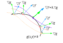
That is, Ńf is parallel to Ńg only if there is a number l for which
Thus, the extrema of f( x,y) subject to g( x,y) = k
must occur at the points which are the solution to the system of equations
We call (1) a Lagrange multiplier problem
and we call l a Lagrange multiplier.
To
solve a Lagrange multiplier problem, we usually solve for l in the
first two equations in (1) to obtain
Once l has been eliminated, we solve for x and y using the
resulting 2 equations in 2 unknowns:
|
|
fx
gx
|
= |
fy
gy
|
, g( x,y) = k |
|
Moreover, if the constraint is a closed curve, then the extrema must occur
at the critical points. Thus, we simply test f( x,y) at the
solutions to (1) in order to identify the extrema of f( x,y) over g( x,y) = k.
EXAMPLE 1 Find the extrema of f( x,y) = xy+14
subject to
Solution: That is, we want to find the highest and lowest points on
the surface z = xy+14 over the circle x2 + y2 = 18:
If we let g( x,y) = x2+y2, then the constraint is g(x,y) = 18. The gradients of f and g are respectively
|
Ńf =
á y, x
ñ and Ńg =
á 2x, 2y
ñ |
|
As a result, Ńf = lŃg implies that y = l2x and x = l2y. Clearly, x = 0 only if y = 0, but ( 0,0) is not
on the circle. Thus, x ą 0 and y ą 0, so that solving for l yields
|
l = |
y
2x
|
and l = |
x
2y
|
Ţ |
y
2x
|
= |
x
2y
|
|
|
Cross-multiplying then yields 2y2 = 2x2, which is the same as y2 = x2. Thus, the constraint x2+y2 = 18 becomes
|
x2+x2 = 18, x2 = 9, x = ±3 |
|
Moreover, y2 = x2 implies that either y = x or y = -x, so that the
solutions to (1) are
|
( 3,3) , ( -3,3) , ( 3,-3) , (-3,-3) |
|
However, f( 3,3) = f( -3,-3) = 23, while f(-3,3) = f( 3,-3) = 5. Thus, the maxima of f(x,y) = xy+14 over x2+y2 = 18 occur at ( 3,3) and ( -3,-3) , while the minima of f( x,y) = xy+14 occur
at ( -3,3) and ( 3,-3) .
Check your Reading: What lines through the origin in the xy-plane contain the critical points in example 1?