Limits along different paths

In single variable calculus, we learn that limits exist only when the limit from the left and right yield the same number. This idea generalizes to functions of 2 variables to say that the limit of f ( x,y ) exists as ( x,y ) approaches ( p,q ) only if the limit of f ( x,y ) along any path through ( p,q ) yields the same value.

Conversely, if the limits along any two paths differ, then the two-variable limit of the function does not exist.

Let's look at an example. Let's consider the limit below along different paths:

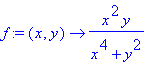
To do so, let's first define the function and the point we are approaching.

> f:=(x,y)->(x^2*y)/(x^4+y^2);
p:=0;
q:=0;

>

Next, let's compute the limit of f along different paths leading to ( p,q ):

> #Limit along the x-axis (i.e., where y=0)
limit(f(x,0),x=0);
#Limit along the y-axis (i.e., where x=0)
limit(f(0,y),y=0);
#Limit along the line y=x
limit(f(x,x),x=0);

>

>

Now let's consider the limit of f along a different path--i.e., along the path y=x

> #Limit along the line y=x^2
limit(f(x,x^2),x=0);

>

Thus, the original limit does not exist. Let's look at the graph of f ( x,y ) as a means of more fully exploring this limit. Let's first consider one of the curves above:

> #Enter a curve through (p,q) in the form y=g(x) or x=h(y)
limit_path:=y=0:
path_range:=x=-1..1:

# Below we construct the graph
surf_plot:=plot3d(f(x,y),x=p-1..p+1,y=q-1..q+1):
parp:=subs(limit_path,[x,y]):
path_plot:=tubeplot([parp[1],parp[2],f(parp[1],parp[2])],path_range,color=blue,radius=0.05):
display(surf_plot,path_plot,axes=normal);

>

Along this path, the limit appears to be 0. However, let's choose a different path

> #Enter a curve through (p,q) in the form y=g(x) or x=h(y)
limit_path:=y=x^2:
path_range:=x=-1..1:

# Below we construct the graph
surf_plot:=plot3d(f(x,y),x=p-1..p+1,y=q-1..q+1):
parp:=subs(limit_path,[x,y]):
path_plot:=tubeplot([parp[1],parp[2],f(parp[1],parp[2])],path_range,color=blue,radius=0.05):
display(surf_plot,path_plot,axes=normal);

>

Notice now that the function values stay above the limit values above. Thus, we can conclude that